I received an assessment after applying for an analytics position with a baseball team. Anyone who knows me knows this would be a dream job in a way, having played softball basically my whole life. I dove right into the assignment, which had the stipulation of only spending 1 - 2 hours on it. I did try to stay within the limits, but the subject matter being one of those magical marriages between personal and professional interests, I continued on afterwards to practice 1) scaling and sampling techniques and 2) creating useful visualizations for the results.
Background
The data were a collection of pitch location data from different minor league baseball games. The goal was to predict whether or not a pitch is a called strike - so I am only given pitches at which the batter did not offer. In theory, calling pitches should only depend on position but until the league embraces the robot umpire revolution, there is always room for human error.
Data Cleaning
The data were already neatly in a CSV so no need for webscraping. I started by just reading the file using Pandas and looking at the column names and data types. Columns are GameID, PitchNumber, Balls, Strikes, PitcherHand, BatSide, PlateHeight, PlateSide, and CalledStrike. So I have unique IDs for each game, pitch number within that game, the count at the time (Balls, Strikes), categorical variables for the pitcher and batter handedness, the pitch location, and the resulting call. I added one feature here, a boolean describing if the pitcher and batter were of the same handedness.
There were only 111 observations having null values in pitch location data of the 62577 pitchers, so I removed those observations. I then used the get_dummies() function in Pandas to turn the PitcherHand and BatSide categorical variables into dummy columns, boolean variables indicating whether or a not a pitcher (batter) is right-handed.
Data Exploration
The CalledStrike column was the dependent variable, and the distribution of calls was somewhat imbalanced (42911 balls, 19555 strikes). This was something I addressed later. Another change I made was the GameID column - it seemed to be a unique string assigned to each game and the data were made of pitch data from 404 unique games. To avoid data leakage, I decided to split the data into train-validation-test sets along game lines. I used the factorize() method to convert the GameIDs into an integer signifying the group (game) from which that observation originated.
Plotting the data using the pairplot functionality in Seaborn allowed me to explore each feature’s individual influence on called strikes, a univariate analysis revealing if features were able to separate the data. Interestingly, the influence on the count is not high - called strikes are called strikes no matter the count - but there is the greatest difference in the classifications when the count has no strikes. Not to say the strike zone changes; with no strikes, batters probably are more likely to take a strike.
Data Analysis
I began by splitting the data into 80/20 train and test fractions along group lines by using the GroupKFold class, setting the number of folds to 5, then breaking out of the loop finding the indices after one iteration. The test fraction was for ultimately determining the best model, while the train fraction was for testing different models.
Those different models varied in the type of scaler and type of sampling. Starting with scaling, as the features were all of the same order of magnitude, I didn’t think it much of a priority. Also, the tree models don’t require scaling, but still it is good practice so I started with the StandardScaler from the preprocessing module in scikit-learn. To address the imbalanced data, I used the imbalanced-learn package, starting with the simple RandomUnderSampler. For classifiers, I tried KNearestNeighbors from scikit-learn, BalancedRandomForestClassifier and EasyEnsembleClasifier from imbalanced-learn, and XGBClassifier from XGBoost. A caveat here is that the BalancedRandomForestClassifier uses a RandomUnderSampler to balance the classes first - but I’d added the sampler in the pipeline already so I think this is akin to using the regular RandomForestClassifier in scikit-learn. I used the RandomizedSearchCV to sample different parameters for the four classifiers; it tries some but not all of the combinations to get a sense of what the best option could be. Finally, for scoring I optimized for precision - basically thinking that I want to be confident in, if wanting a pitch to be a strike, it actually is. In other words, minimizing false positives.
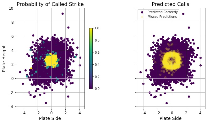
The results of this first fitting showed that the best classifier was KNearestNeighbors, and even after trying a full GridSearchCV on different number of neighbors, the best score came from just two neighbors. Looking at incorrectly predicted pitches, they tended to land on the periphery of the strike zone - borderline calls. It as if the predictions were suffering from too much data: this is where calls are likely incorrect in a game, so a KNN fit with only 2 nearest neighbors heavily dependent on pitch location (information I’d gleaned during a fitting using the BalancedRandomForestClassifier) could easily be influenced by previous wrong calls in the training data.
With that in mind, I looked back into the undersampling techniques. I tested two additional options from imbalanced-learn that specifically undersample majority data near the decision boundary, TomekLinks and NearMiss. I also tried a few of the other scaling methods: MinMaxScaler, MaxAbsScaler, and PowerTransformer. I repeated the same methodology as before, using the RandomizedSearchCV and several options for parameters, optimizing for precision.
Before I give the results, I’ll note that not all undersampling techniques are alike. The RandomUnderSampler allows the user to choose the final class ratio, defaulting to 50/50. TomekLinks only removes those points (default removes those from the majority aka overrepresented class) that are classified as Tomek’s links, so those whose nearest neighbor is of the opposite class. This may not balance a dataset, so to reach that 50/50 ratio, the user then needs to employ a second sampling technique. NearMiss version 1 defaults to removing the majority points with the shortest average distance to N (default, N = 3) nearest neighbors of the opposite class. Like RandomUnderSampler, will default to balancing the classes. With that said, in this analysis, I followed the TomekLinks undersampler with a RandomUnderSampler to balance the classes.
The best score came from a combination of the MinMaxScaler, the NearMiss sampler, version 1, and the KNN classifier, outperforming my previous best by 0.033. I then fed this pipeline into GridSearchCV, allowing both the number of nearest neighbors for both NearMiss and KNN to vary and landed on a slightly better precision score using just one nearest neighbor for the NearMiss undersampling. This step removed majority class points closest to a minority class until the two were balanced. With this final result, I achieved a precision score on the test data of 0.8743.
Out of curiosity, I went back and re-fit just the location data (PlateHeight and PlateSide columns). While the results from combinations of scaler, sampler, and classifier sometimes result in better or worse precision scores on the validation sets, the best cross-validated result is ~0.014 worse than the best from using all the features. Again, I fed the best estimator (StandardScaler, NearMiss sampler, version 1, and KNN classifier) into GridSearchCV and got the same results for best parameters: one nearest neighbor for NearMiss and two for KNN. This classifiers yielded a precision score of 0.8834 on the test data, better than that from using all the data.
Results
In real numbers, the classifier fitted with all features incorrectly predicted strikes on 395 pitches, while using location data only 361 pitches were wrongly predicted strikes. This was over a test data set of 81 games, so less than five per game in both cases.
| predicted | |||
|---|---|---|---|
| False | True | ||
| actual | False | 8186 | 395 |
| True | 1173 | 2748 | |
| predicted | |||
|---|---|---|---|
| False | True | ||
| actual | False | 8220 | 361 |
| True | 1187 | 2734 | |
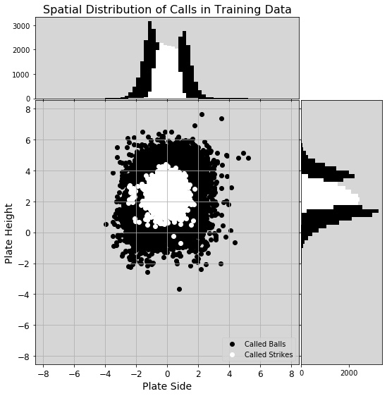
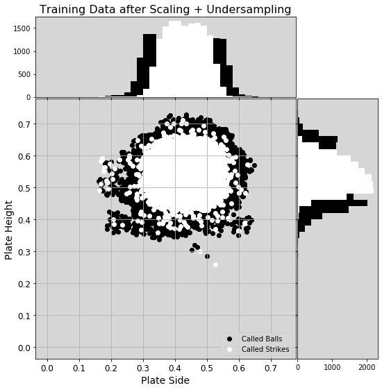
Just to better understand the false positives and false negatives, I looked only at their data. Interestingly, there are more missed predictions on one side of the plate (the mean would be zero if equally distributed laterally). The training data was asymmetric before scaling and undersampling (see figure), but those steps seemed to correct the lateral asymmetry. Still there remained a population of called strikes on the left side of the plot (I’m assuming outside to a right-handed batter, though I wasn’t told how the pitch location numbers mapped to real space), and their presence in the training data contributed to the missed calls outside.
In conclusion, how did the classifier perform? By optimizing for precision, I was able to achieve fewer than five false positives per game - so each team has less than 2.5 actual strikes be called balls. From the batter’s perspective, however, the number of false negatives is much higher, with ~14.5 false negatives per game. Had I optimized for F-score instead of precision, it’d have been fairer for batter and pitcher alike. Also, if I’d been able to train with better data (correctly called balls and strikes, perhaps pulled from here), there’d have been fewer missed pitches at the strike zone boundary. That site produces accuracy scores for each Major League Baseball umpire, where umpires’ average accuracy scores across this past season range from 91.3% to 95.7% - accuracy of calls against a universal strike zone. My classifier, while not optimized for accuracy, achieved accuracy scores of 87.5% and 87.6%, so not quite up to MLB standards. Maybe these umpires responsible for the calls in my training data are in the minors for a reason?