In an attempt to data science my way to solutions to the world’s problems, I tried to predict results from professional men’s tennis. More specifically, I used existing rankings and statistics to determine if a given player would make the round of 16 (R16) of a Grand Slam tournament. This wasn’t even for gambling purposes - I’m too cheap to gamble - but the motivation to see my favorite players in person. Ticket prices increase with each round and go on sale before the tournament starts, so it’s a gamble to spring for pricey later round seats without knowing who the players will be. Knowing with greater certainty that my favorites would be playing, perhaps I’d be more willing to spend more.
Background
The four annual Grand Slams are the pinnacle(s) of the professional tennis calendar, as much as one can have four pinnacles. There are smaller tournaments throughout the year but the Australian Open, the French Open (Roland Garros), Wimbledon, and the US Open feature the largest purses and draws on the tour. Competitors must navigate a field of 128 players, 104 of which come from the top of the ATP rankings. The remaining 24 come from qualifying rounds or wildcard exemptions. Further, the top 32 of those are seeded and given an easier path, in theory, to prevent the the top two meeting before the finals, the top four before the semifinals, and so on. ATP rankings are a 52-week rolling point total that rewards both performance and tournament difficulty. The tournament seedings follow ATP rankings except for at Wimbledon, where they prioritize recent grass court performance. This in itself has been a controversial topic but is outside the scope of this analysis.
Data Collection
Data were from this Git repository that lists matches of all three levels of professional tennis. I only needed the top two tiers: those with ATP-level matches and those with Challenger Tour and qualifier matches. I focused from 2015 to 2020, through the 2020 Australian Open. Since I was looking at match stats from previous weeks, I also needed the 2014 matches.
Data Collation on PostgreSQL
For the most part, the column labels and data types are consistent from year to year, aiding in agglomerating the results. One caveat I’ll note is the tourney_date column is not the date the match actually was played but rather the official start of the tournament, which came into play later.
I used the information schema from one table as a key to find the mismatched data types in the other tables. The incompatible data types usually involved non-numeric designations in the seed columns, which I moved to the categorical entry column instead. Once converted, I combined all of the files into one giant table. This made searching for past data easier as I didn’t have to loop through different filenames but wouldn’t be efficient if combining decades of data, as the table size grows unwieldy.
Data Selection on PostgreSQL
I needed to find the main draws from all the Grand Slams, who of those players survived to the R16, and then the matches everyone played in the six weeks prior. I chose the six weeks as an arbitrary interval to suss out any players on a “hot streak.”
The aforementioned tourney_date issue caused problems when collecting previous matches by dates:
- Grand Slam qualifying round (Q1, Q2, Q3) matches were labeled with the same tourney_date as the start of the main draw despite being played the week before
- matches played deeper in tournaments thus within the time window could be missed if the tourney_date lies outside the window
I had to ignore the latter issue; I didn’t want to look up the precise dates of all the matches played. For the former, I just had to make sure qualifying rounds were included in the previous matches table. It culminated in left joins between the main draw and the prior matches that resulted in two tables: one with all of the players in the main draws of the Grand Slams, and the other with the previous matches they played.
Analysis and Feature Engineering
I moved the PostgreSQL tables to a Jupyter notebook and created new features to include stats from the previous matches. Those features included:
- number of matches played
- number of wins in those matches
- number of those matches that were on the same surface as the upcoming Grand Slam
- the number of those matches that were in each level (from high to low, G for Grand Slams, M for Masters 1000 ATP events, A for other ATP-level events, and C for Challenger Tour levels)
- whether or not the Grand Slam was in the player’s home country
Service game stats for those previous matches included:
- number of aces normalized by service points
- number of double faults normalized by service points
- number of first serves won normalized by service points
- number of first serves made normalized by service points
- number of second serves won normalized by service points
- number of break points faced normalized by service points
- number of break points saved normalized by service points
- mean ranking and points total of the Grand Slam entrant
- mean ranking and points total of his previous opponent(s)
Some of the features resulted in NaN values that needed to be replaced. If the player hadn’t played in any events leading up to the Grand Slam, he has no match-specific stats so I replaced those NaN values with zeroes. Similarly, players without prior match stats had NaN values for mean ranking and points totals for himself and his previous opponents. His ranking and points total were probably very similar to the ranking and points total he had at the start of the Grand Slam, so I dropped those. For opponent rankings, I couldn’t think of a proper way to fill NaNs so I dropped that feature but filled the opponent mean points NaNs with zeroes.
Some of the player-specific details about Grand Slam entrants also had NaNs. Only the top 32 players are seeded but setting the rest to zero seemed both wrong and oversimplified. I instead used the rankings and points totals to assign seeds to the rest of the draw. I followed the same methodology for unranked players, sorting by points totals then assigning one greater than the maximum ranking in the draw. If players had NaNs as their points totals, I replaced those with zeroes.
The player entry column is mostly NaNs but categorical, so I turned that into a dummy variable. I also changed the player hand column to a dummy variable after replacing the unknown values (U) with the more likely right-handed (R).
I used the SimpleImputer from scikit-learn to fill missing player heights with the average player height in a given Grand Slam draw. Since I separated train/validation/test sets by tournament, I avoided data leakage by imputing player heights along tournament lines also.
Fitting Estimators
I split the data into train/validation/test sets along tournament lines, ending up with 25% of the data (five tournaments) as the test set. I wanted to split along tournament lines to avoid having one Grand Slam (e.g., all US Opens) to be entirely in the test set. I used GroupKFold from scikit-learn with the default five folds that split the remaining 75% into train and validation sets along group (here, tournament) lines. I utilized the RandomOverSampler from imblearn since the classification results were imbalanced (16 True, 112 False). I also used the StandardScaler in the pipeline, which isn’t necessary for tree-based models but standardizes feature importance coefficients, which is helpful for model interpretation.
I tried a handful of models and hyperparameters through GridSearchCV with the five folds of GroupKFold, optimizing for precision, recall, and f1 separately. In hindsight, overkill, but I was running the fittings before having decided the proper scoring metric. I ended up with three best estimators for each of eight models, then compared them by looking at their ability to correctly predict the R16 qualifiers in my test set. I used the predict_proba method to find the probability of a player in the main draw to make the R16, then assigned the top 16 probable candidates as the predicted 16. Always predicting 16 Trues led precision to equal recall (and f1, as their harmonic mean). It was possible to have multiple players with the same odds, so in those cases I used the minimum of precision or accuracy to compare different estimators as to not artificially inflate the score when predicting > 16 Trues per tournament. In the end, the XGBoost model with hyperparameters optimizing recall yielded the best precision and/or recall.
| optimized for precision | optimized for recall | optimized for f1 score | |
|---|---|---|---|
| KNN | 0.235294 | 0.556818 | 0.451613 |
| Logistic | 0.6125 | 0.65 | 0.6125 |
| Decision Tree | 0.556522 | 0.568421 | 0.556522 |
| Random Forest | 0.6125 | 0.593023 | 0.625 |
| Support Vector Machine | 0.45 | 0.6 | 0.6 |
| Polynomial SVM | 0.5 | 0.5625 | 0.6125 |
| Extra Trees | 0.65 | 0.55 | 0.6125 |
| XGBoost | 0.6375 | 0.666667 | 0.6375 |
The ATP Tour was dominated by the top seeds, at least in terms of championships, from 2003 to 2020. It made sense to see how well the tournament seeds predict the R16 qualifiers, since its entire purpose is to get the top seeds to the later rounds. I used the top 16 seeds as the predicted True, calculated the precision and recall (here, equal), and found that the seeds alone outperformed my classifier at 0.7125. Frustrating!
Reducing Features and Refitting Estimators
Motivated by my classifier underperforming the simple seedings, I wondered if the inclusion of too many features was increasing the variance in my predictor while sacrificing any benefits those weaker features were imparting. I decided to reduce my feature set via BorutaPy, a Python implementation of the Boruta feature selection package.1 I retained 10 of the 26 features and repeated the GridSearchCV as before and found the best classifier was a logistic regression, and it slightly outperformed the XGBoost classifier at 0.6875.
| optimized for precision | optimized for recall | optimized for f1 score | |
|---|---|---|---|
| KNN | 0.457143 | 0.456311 | 0.473684 |
| Logistic | 0.6875 | 0.65 | 0.6875 |
| Decision Tree | 0.556522 | 0.538462 | 0.556522 |
| Random Forest | 0.65 | 0.576577 | 0.6 |
| Support Vector Machine | 0.525 | 0.65 | 0.6625 |
| Polynomial SVM | 0.5875 | 0.6125 | 0.6625 |
| Extra Trees | 0.6625 | 0.666667 | 0.6625 |
| XGBoost | 0.625 | 0.666667 | 0.6125 |
I wanted to try another method of reducing variance that I’d seen. It’s been shown that, for some cases, the benefits of feature reduction can be matched with bagging while avoiding the computational cost of feature reduction.2 In this case, I don’t have a prohibitive number of features but I wanted to try it regardless. I chose the best estimator from the full feature set and ran GridSearchCV to determine the proper number of estimators, feature subsets, and sample subsets. Indeed, the bagged XGBoost classifier matched the precision of the reduced feature set.
| optimized for precision | optimized for recall | optimized for f1 score | |
|---|---|---|---|
| XGBoost | 0.6375 | 0.666667 | 0.6125 |
| Bagged XGBoost | 0.675 | 0.675 | 0.675 |
I then repeated the bagging optimization for the reduced feature set using the optimized logistic regression.
| optimized for precision | optimized for recall | optimized for f1 score | |
|---|---|---|---|
| Logistic | 0.6875 | 0.65 | 0.6875 |
| Bagged Logistic | 0.7 | 0.6875 | 0.7 |
Bagged, the best estimator from the reduced feature set gets closer still to the performance of the top 16 seeds.
Results
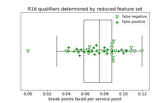
I wanted to understand which players my estimator was misclassifying to better understand its performance. Using the best estimator from the reduced feature set as my predictor, I began plotting the true positives, false positives, and false negatives of each feature individually, starting with the feature with the largest coefficient from the base (logistic) estimator. Since the features were scaled, the absolute value of the coefficients give a measure similar to feature importance. The most influential features were the seed, ranking, and ranking points; plots of these showed clear delineation between true positives, false positives, and false negatives. Compared to the actual R16 qualifiers that shown on the box plots, the false negatives fell beyond the 75th percentile of the true positives whereas the false positives were understandably located closer to the true positives. Comparatively, the false negatives and false positives from match stats-based features (break points, first serves won, double faults, and opponent ranking points) were more randomly distributed onto the true positives.
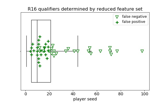
It seemed that any influence from the match-based stats was overridden by the seeding and ranking. Using those together with the match-based stats didn’t reveal any of these underdog R16 qualifiers, so I reran the analysis with only the stats affected by matches in the previous weeks. While I didn’t expect the results to outperform the prior estimators, I hoped it would find more players outside the top 16 seeds who were predicted to reach R16. It did find three additional R16 qualifiers outside the top 16, but it also cost many more false positives outside the top 16.
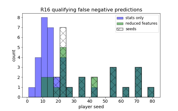
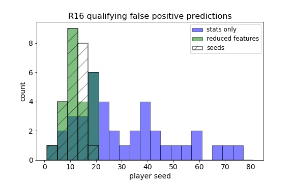
So in the end, the tournament seeding just slightly outperformed the reduced feature set, which itself was heavily dependent on the tournament seeding. It isn’t to say that recent match successes were irrelevant in this data, but they weren’t enough to propel an underdog all the way to the round of 16. As for the lofty goal of guessing whether a given player would make this round, the chances are high that if he is in the top 16 seeds, he’ll advance. Outside those, someone in the next 8 seeds might have a chance, especially if he has dominant serve statistics in his previous matches. Indeed, being able to hold one’s serve is key to success in any tennis match, and those who excel at it are more likely to advance to the later rounds of any tournament.
References
-
Kursa, M., & Rudnicki, W. (2010). Feature Selection with the Boruta Package. Journal of Statistical Software, 36(11), 1 - 13. doi: http://dx.doi.org/10.18637/jss.v036.i11 ↩
-
Munson M.A., Caruana R. (2009) On Feature Selection, Bias-Variance, and Bagging. In: Buntine W., Grobelnik M., Mladenić D., Shawe-Taylor J. (eds) Machine Learning and Knowledge Discovery in Databases. ECML PKDD 2009. Lecture Notes in Computer Science, vol 5782. Springer, Berlin, Heidelberg. doi: http://dx.doi.org/10.1007/978-3-642-04174-7_10 ↩